| ddplot | ||||
| Visualization of 3D dislocation strain fields 2D differential displacement maps | ||||
| Screenshots | Download | File formats | Contact | |
This program visualizes dislocations in crystals using the so-called differential displacement maps. If dislocations are present in the crystal, the atoms close to its core are displaced from their positions in the ideal crystal. The change in the separations of neighboring atoms is depicted by arrows whose lengths correspond to the magnitudes of the changes of their separation relative to their distance in the ideal crystal.
The main features implemented in ddplot are:
Screenshots
Click on the pictures below to see their actual size.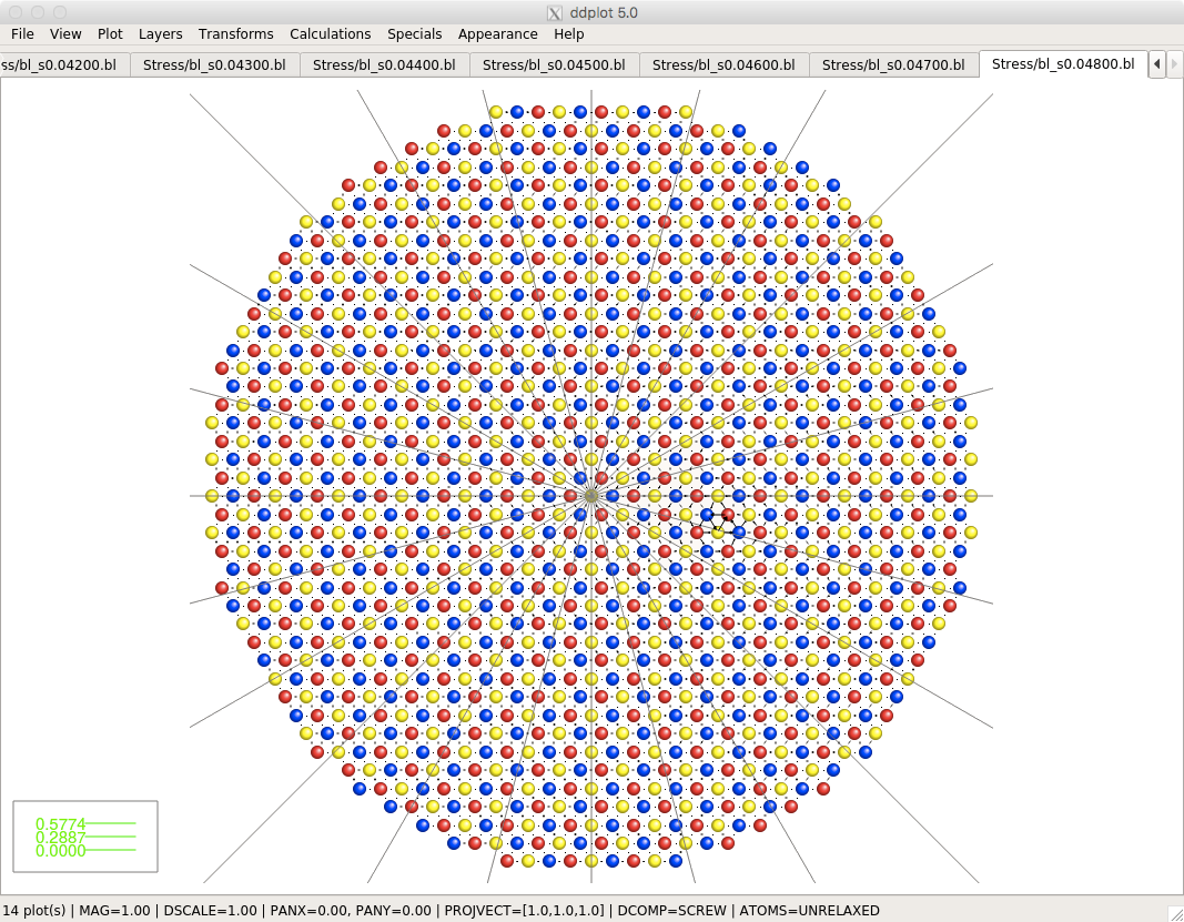 Snapshot of ddplot showing a block of Mo atoms with a 1/2[111] screw dislocation that has moved from the center by the action of applied shear stress parallel to the slip direction. The arrows correspond to the screw displacements perpendicular to the plane of the figure. The gray lines are traces of planes that make angles 0, 15, 30, 45, 60, 75 and 90 deg with the (-101) plane. |
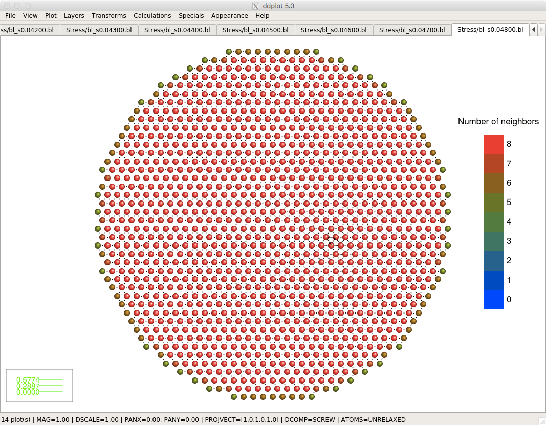 Snapshot of Mo atoms in the bcc structure showing the atoms colored according to the number of neighboring atoms (see the color bar on the right). The list of atomic planes is shown on the left (they can be turned on and off to make calculations only for a given slab of atoms). |
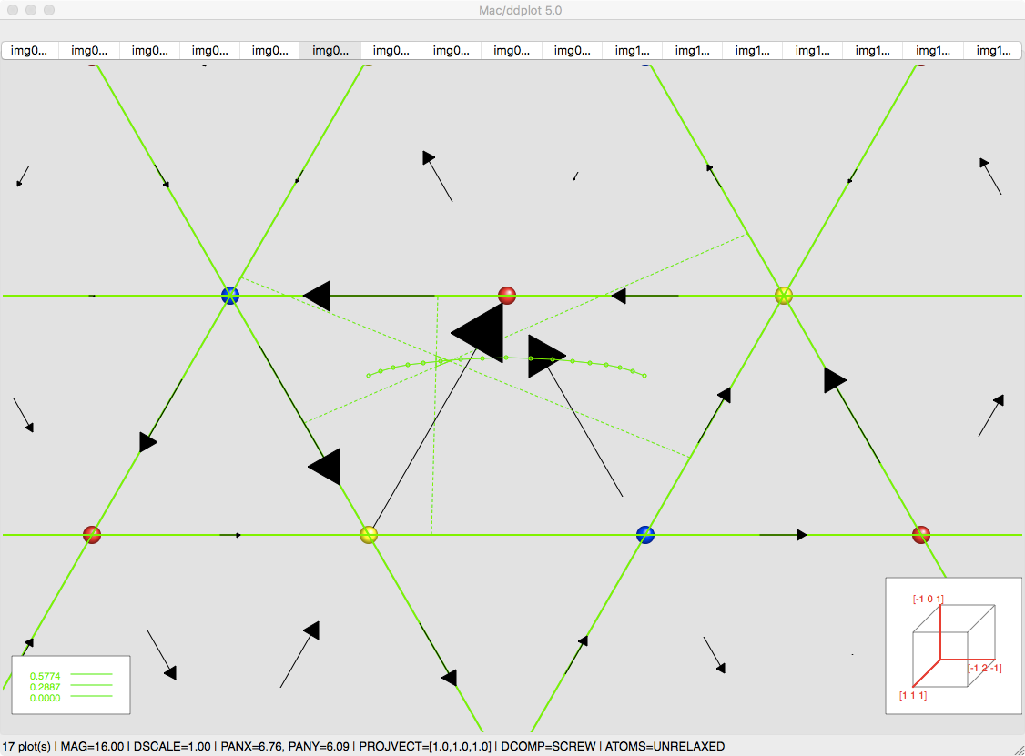 In the version 5.0+ ddplot allows to find the dislocation position and dislocation pathways, for example from a series of atomic configurations obtained by the Nudged Elastic Band method. This snapshot shows such calculation for 17 atomic blocks of bcc Mo. The little green triangles are approximations of dislocation positions. The green curve is the calculated dislocation pathway. |
Download
version 5.2 (released October 24, 2022)
 Windows 7/8/10 (64bit) Windows 7/8/10 (64bit) |
ddplot-5.2-win64.zip | unzip and run ddplot.exe |
 Source code Source code |
ddplot-5.2-src.tar.gz | compile with Qt5 library |
| Default settings | .ddplot | Loaded on startup. Store in your home directory and edit with a text editor. |
version 5.1 (released June 23, 2020)
| Windows 7/8/10 (64bit) |
ddplot-5.1-win64.zip | unzip and run ddplot.exe |
 Mac OS X (64bit) Mac OS X (64bit) |
ddplot-5.1-mac64.dmg | tested on macOS 10.13.6 High Sierra |
 Linux (Ubuntu 64bit) Linux (Ubuntu 64bit) |
ddplot-5.1-linux64.tar.gz | x86_64, compiled with Qt 5.15.0, tested on Ubuntu 20.04 LTS |
| Source code |
ddplot-5.1-src.tar.gz | compile with Qt5 library |
| Default settings | .ddplot | Loaded on startup. Store in your home directory and edit with a text editor. |
You can also get the latest sources from github as:
git clone https://github.com/romangroger/ddplot.git ddplot
Follow the instructions there to compile and run.
File formats
Following is a list of file formats that are readable by ddplot. If you want to use this code for plotting, you are supposed to prepare your data in one of the supported formats. The only format that ddplot uses for saving is the internal .dd format that whose complexity will evolve in future releases to accommodate all possible information required for effective plotting of the differential displacement maps. The underlined words are keywords and must appear as written below..xyz format
This is the most trivial format that does not contain any information about the orientation of the block, periodicity and the like. It is entirely up to the user of ddplot to remember these parameters.
ninit number of atoms in the initial structure
title_init
el1 x(1) y(1) z(1)
el2 x(2) y(2) z(2)
: : : : coordinates of atoms in the initial configuration
: : : : (usually unrelaxed ideal lattice)
eln x(n) y(n) z(n)
nrel
title_rel
el1 x(1) y(1) z(1)
el2 x(2) y(2) z(2)
: : : : coordinates of atoms in the relaxed
: : : : configuration (relaxed structure)
eln x(n) y(n) z(n)
BVECT bx by bz Burgers vector of screw dislocation (if any)
.plt format
This is an old format used in one of our simulation codes. Note, that the number of atoms in the relaxed configuration should be identical to that in the perfect lattice. The relaxed configuration is usually obtained by stressing a perfect crystal, where the initial positions of atoms correspond to the perfect lattice.
nrel number of atoms in the relaxed configuration
z(1)
z(2)
: z-positions of atoms in the relaxed
: configuration
z(nrel)
x(1) y(1) zlayer(1)
x(2) y(2) zlayer(2)
: : : (x,y) positions of atoms in the
: : : relaxed configuration
x(nrel) y(nrel) zlayer(nrel)
ninit number of atoms in the perfect lattice
z(1)
z(2)
: z-positions of atoms in the perfect lattice
:
z(nrel)
x(1) y(1)
x(2) y(2)
: : (x,y) positions of atoms in the perfect
: : lattice
x(ninit) y(ninit)
0 unused, don't ask me why
xperiod
yperiod periodicity in the x, y, z directions
zperiod
CORE { xpos; ypos } (x,y) position of the screw dislocation
If the block does not contain any screw dislocation, simply omit the last line.
.bl format
This is another format from the same simulation code that we are using. The format is a bit complicated and is not supposed to be used any more. It is left in ddplot only for the sake of quick visualization of the results of our simulations.
LEN
xlen ylen zlen x, y and z size of the block
LATPAR
latpar lattice parameter
ND
nd number of active atoms
D
x(1) y(1) z(1) elem(1)
x(2) y(2) z(2) elem(2) coordinates of active atoms in the
: : : : relaxed configuration and the name
: : : : of the element, e.g. Mo
x(nd) y(nd) z(nd) elem(nd)
NINERT
ninert number of inert atoms
DINERT
x(1) y(1) z(1) elem(1)
x(2) y(2) z(2) elem(2) coordinates of inert atoms in the
: : : : relaxed configuration and the name
: : : : of the element, e.g. Mo
x(ninert) y(ninert) z(ninert) elem(ninert)
UNRLD
x(1) y(1) z(1) elem(1)
x(2) y(2) z(2) elem(2) coordinates of atoms in the
: : : : perfect lattice and the name
: : : : of the element, e.g. Mo
x(nunrld) y(nunrld) z(nunrld) elem(nunrld) nurld=nd+ninert
In our simulations, the block is usually divided into two parts. Outer part of the (x,y) plane contains inert atoms into which we apply anisotropic displacements corresponding to a given stress field. The inner part then contains active atoms whose position is obtained by minimization. In the relaxed configuration, the force on each atom is essentially zero.
.dd format
This is the internal ddplot's format that contain all possible information about the block, including the orientation of the block, positions of dislocations, periodicity, etc. Each block starts with a header that is written below in capital letters. Comments begin with '#' and are ignored by ddplot. Number of spaces between each number in a row and between lines is arbitrary.
CSYS orientation of the block given by three
x1 y1 z1 vectors defined in the cube coordinate system
x2 y2 z2 [100], [010], [001]
x3 y3 z3
PERIOD
xperiod yperiod zperiod periodicity along x, y and z
DISLO_CENTER
xpos ypos (x,y) position of the screw dislocation
NUM_UNREL
ninit number of atoms in the perfect lattice
COOR_UNREL
x(1) y(1) z(1) elem(1)
x(2) y(2) z(2) elem(2) coordinates of atoms in the
: : : : perfect lattice and the index
: : : : of the element of this atom
x(ninit) y(ninit) z(ninit) elem(ninit) (count from 0)
NUM_REL
nrel number of atoms in the relaxed configuration
COOR_REL
x(1) y(1) z(1)
x(2) y(2) z(2) coordinates of atoms in the relaxed
: : : configuration
: : :
x(nrel) y(nrel) z(nrel)
The mandatory fields are NUM_UNREL, COOR_UNREL, NUM_REL, COOR_REL and PERIOD.
Contact
Roman Gröger (email: click here)To keep you updated about new versions of ddplot, send me your e-mail and I will add you into the ddplot mailing list. I will be glad to hear about your experience with ddplot, your suggestions but also criticism. If you have some nice figures from ddplot, please, send me .JPG or .GIF to put them here as screenshots.